Starbucks Capstone Project Report
Thien Ngan Doan
Udacity ML Engineer Nanodegree
Jan 2021
I. Overview
This Starbucks Capstone project is part of the Udacity Machine Learning Engineer Nanodegree. Udacity partnered with Starbucks provide a real-world business problem and simulated data that mimics their customer behavior.
Starbucks has a reward program that allows customers earning points for purchases. There is also a phone app for their reward program where they send exclusive personalized offers based on customers spending habits.
This project is focused on tailoring personalized offers to the customers who are most likely to use them. The Machine Learning terminology for this is propensity modeling. Propensity models are often used to identify the customers most likely to respond to an offer.
With the well-organized related data, machine learning becomes a useful tool to improve revenues for business but also to offer better services.
With the smartphone revolution, there are many applications for business services, and those apps collect insightful data about the user behaviors browsing the app that help predicting their needs and provide them the right offers.
This project is a wonderful example, it is a case of study to analyze related data provided by Starbucks and Udacity to make decisions for sending offers to the client.
My goal is analyzing this type of data to apply the same ideas in other similar projects in real productions.
II. Problem Statement
We want to determine the classes of customers which complete valuable offers to success in this project we concentrate on two types of offer: bogo and discount.
Some customers do not want to receive offers and might be turned off by them, some do not view the offers and maybe some fulfill the offer although they never view the offer.
III. Evaluation Metrics
In the first step, as a prototype model, we use only accuracy score metric for sklearn Logistic Regression models.
In the second and third steps, with the powerful Autogluon Tabular we use many types of compatible metrics, such as the scores of accuracy, balanced accuracy, roc_auc, f1, precision, recall.
IV. Data Exploration
We use the dataset provided by Starbucks and Udacity. The
data consists of 3 files containing simulated data that mimics customer
behavior on the Starbucks Rewards mobile app.
1. portfolio.json: information about the offers,
2. profile.json: information about the customers,
3. transcript.json: info about customer purchases and relationships with the offers.
We read all 3 files and transform into the pandas DataFrame type for efficient processing data.
Process data from portfolio.json:
We transform data in this file into a pandas DataFrame port_df for processing data. First here, there exist 10 rows, 6 columns, and no null values .
RangeIndex: 10 entries, 0 to 9
Data columns (total 6 columns):
# Column Non-Null Count Dtype
--- ------ -------------- -----
0 reward 10 non-null int64
1 channels 10 non-null object
2 difficulty 10 non-null int64
3 duration 10 non-null int64
4 offer_type 10 non-null object
5 id 10 non-null object
dtypes: int64(3), object(3)
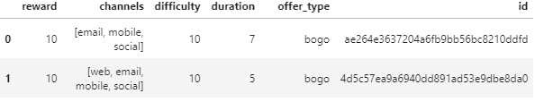
- id: is string type, we replace by number to have good view data, we have 10 ids got number from 0 to 9. We change name "id" into a meaningful name "offer_id".
- channel: has 4 values email, web, mobile, social, we write a small function to encode to 4 binary columns.
def encode_df_col(df, col):
'''
df: DataFrame
col: an encoded column of df
'''
sep_cols =
pd.get_dummies(df[col].apply(pd.Series).stack()).groupby(level=0).sum()
return pd.concat([df,
sep_cols], axis=1)
- reward: compatible value reward of the offer.
- difficulty: the minimum amount spending to have the compatible reward. We change "difficulty" into a meaningful name "min_spend"
- duration: effective time of the offer.
- offer_type: 3 types of "bogo", "discount", and "informational", we use our function to encode 3 columns " bogo", "discount", and "informational".
- We write a function to move column 'offer_id" to the first columns of this dataframe for a good view.
def move_col_first(df, col_name):
'''
df: pandas
DataFrame
col_name:
column is moved to the first column in df
'''
vals =
df.pop(col_name)
df.insert(0, col_name, vals)
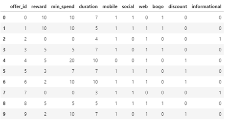
- We remove the columns "channels", "offer_type", "email". The "email" value is always a constant 1, so it is not useful for our research.
RangeIndex: 10 entries, 0 to 9
Data columns (total 10 columns):
# Column Non-Null Count Dtype
--- ------ -------------- -----
0 offer_id 10 non-null int64
1 reward 10 non-null int64
2 min_spend 10 non-null int64
3 duration 10 non-null int64
4 mobile 10 non-null uint8
5 social 10 non-null uint8
6 web 10 non-null uint8
7 bogo 10 non-null uint8
8 discount 10 non-null uint8
9 informational 10 non-null uint8
dtypes: int64(4), uint8(6)
Now a quick look of our port_df dataframe:
Process data from profile.json
Here, there exist 17,000 customers with related information: gender, age, id, become_memger_on, and income. We examine each field later.
RangeIndex: 17000 entries, 0 to 16999
Data columns (total 5 columns):
# Column Non-Null Count Dtype
--- ------ -------------- -----
0 gender 14825 non-null object
1 age 17000 non-null int64
2 id 17000 non-null object
3 became_member_on 17000 non-null int64
4 income 14825 non-null float64
dtypes: float64(1), int64(2), object(2)
- "id": is the customer id, we change it into meaningful name customer_id, and we change its values from a long string to an integer number value to have a good view and easy to process.
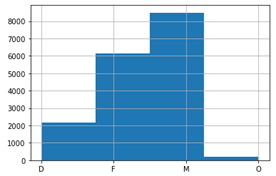
- "gender": here, there exist 3 types F, M, O (Female, Male, Other) and there are null values in this column, we fill the null value by D (Difference) to have full meaning data of gender, after that we encode into 4 other binary columns F, M, O, and D.
Number of null value: 2175
M 8484
F 6129
O 212
Name: gender, dtype: int64
After fill the null value by D, the histogram of gender is as following:
- "age": we will return to parse this values when we examine the combined data to fine the relationship with offers. There is no null value here, but people that do not declare gender set age 118.
prof_df['gender'][prof_df['age'] == 118].unique()
array(['D'], dtype=object)
- "income": its values are from 30,000 to 120,000 and there are 2175 null values.
Number of null income: 2175
count 14825.000000
mean 65404.991568
std 21598.299410
min 30000.000000
25% 49000.000000
50% 64000.000000
75% 80000.000000
max 120000.000000
Name: income, dtype: float64
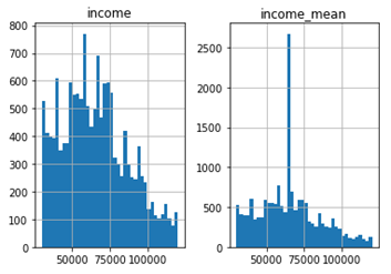
Here is the histogram of income values.
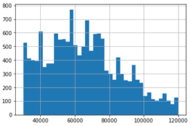
We have many methods to fill in the null values to utilize these data. Now we display two popular methods:
1. mean value:
# Try setting mean value
for null income
mean_inc = round(prof_df['income'].mean(), -3)
prof_df['income_mean'] = prof_df['income'].fillna(mean_inc)
# Histograms
prof_df[['income_mean', 'income']].hist(bins=40)
2. random values in the range of min and max
We write some code to implement this null values filling.
max_inc = max(prof_df['income'].dropna())//1000
min_inc = min(prof_df['income'].dropna())//1000
null_income_indexs =
prof_df['income'].isnull()
new_incomes =
(np.random.randint(min_inc, max_inc, size=sum(null_income_indexs))*1000).tolist()
prof_df['income_rand'] = prof_df['income'].copy()
indexs = []
i = 0
for k, val in enumerate(null_income_indexs):
if val == True:
indexs.append(k)
prof_df['income_rand'][k] = new_incomes[i]
i += 1
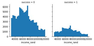
# Histograms
prof_df[['income_rand', 'income']].hist(bins=40)
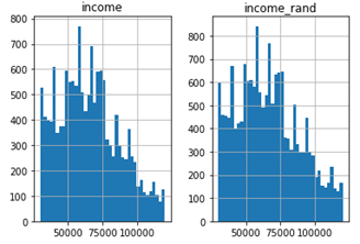
Compare two plots, we see that the income_rand histogram is similar to the original income one. So, we choose the income_rand values for next steps.
- " became_member_on": datetime that the customer was a member. We change the name into a meaningful name 'time_on'.
We move the column customer_id to the first position to have a good order and remove the columns income and income_mean to have a neat and useful data for next steps. Summarize our changes.
RangeIndex: 17000 entries, 0 to 16999
Data columns (total 9 columns):
# Column Non-Null Count Dtype
--- ------ -------------- -----
0 customer_id 17000 non-null int64
1 gender 17000 non-null object
2 age 17000 non-null int64
3 time_on 17000 non-null datetime64[ns]
4 income_rand 17000 non-null float64
5 D 17000 non-null uint8
6 F 17000 non-null uint8
7 M 17000 non-null uint8
8 O 17000 non-null uint8
Process data from transcript.json
Here, there exist 306,534 purchases with 4 columns with information related to the offers and customers.
RangeIndex: 306534 entries, 0 to 306533
Data columns (total 4 columns):
# Column Non-Null Count Dtype
--- ------ -------------- -----
0 person 306534 non-null object
1 event 306534 non-null object
2 value 306534 non-null object
3 time 306534 non-null int64
dtypes: int64(1), object(3)
1. person: this is customer_id in profile data, we substitute it by the name and the numeric value of customer_id.
2. event: there are 4 types of event.
# Examine the event data
tran_df['event'].unique()
array(['offer received', 'offer viewed', 'transaction', 'offer completed'],
dtype=object)
We encode event into 4 binary columns offer_received, offer_viewed, offer_completed, and transaction.
3. value: this is a complicated field; each value is a dictionary data. Write some code, we find there are four types of value data:
{'reward', 'offer id', 'offer_id', 'amount'}
Examine real data, 'offer id' and 'offer_id' are the same, it contain the offer_id in portfolio data. Here we do not know exactly what is the amount, because there is not a clear explain in the document, but it may be useful for our prediction models.
We encode this column into three columns offer_id, amount, and reward. Write some code, we can read the values in reward column, we see that sometime they do not record the reward value as in portfolio, so we remove this column to get the data consistency, because the offer_id implies the reward value.
{3: [0, 5], 4: [0, 5], 9: [0, 2], 6: [0, 2], 1: [0, 10], 8: [0, 5], 5: [0, 3], 2: [0], 0: [0, 10], 7: [0]}
4. time: time in hours since start of test. The data begins at time t = 0.
After processing and cleaning the data, moving customer_id to the first column, we have the dataframe info as following:
RangeIndex: 306534 entries, 0 to 306533
Data columns (total 8 columns):
# Column Non-Null Count Dtype
--- ------ -------------- -----
0 customer_id 306534 non-null int64
1 time 306534 non-null int64
2 offer_completed 306534 non-null uint8
3 offer_received 306534 non-null uint8
4 offer_viewed 306534 non-null uint8
5 transaction 306534 non-null uint8
6 offer_id 306534 non-null int64
7 amount 306534 non-null float64
dtypes: float64(1), int64(3), uint8(4)
Combine data from 3 above dataframes
First we combine data from profile and transcript on value customer_id.
# Merge tran_df and prof_df
data = pd.merge(tran_df, prof_df, on='customer_id')
Second we combine new data with portfolio data on value offer_id.
# Merging on 'offer_id'
data = pd.merge(data, port_df, on='offer_id', how='left')
Process combined data
There are null values in new combined data:
reward 138953
min_spend 138953
duration 138953
mobile 138953
social 138953
web 138953
bogo 138953
discount 138953
informational 138953
These null values attached with the false offer_id 10 (informational transaction) when we process the transaction data.
# Find sample null value
data['offer_id'][data['bogo'].isnull()].value_counts()
10 138953
Name: offer_id, dtype: int64
We can remove all 138953 data rows of offer_id 10.
We change column name offer_comleted as success to have a meaningful name and move it to the first position in dataframe.
Int64Index: 167581 entries, 0 to 306532
Data columns (total 25 columns):
# Column Non-Null Count Dtype
--- ------ -------------- -----
0 success 167581 non-null uint8
1 customer_id 167581 non-null int64
2 time 167581 non-null int64
3 offer_received 167581 non-null uint8
4 offer_viewed 167581 non-null uint8
5 transaction 167581 non-null uint8
6 offer_id 167581 non-null int64
7 amount 167581 non-null float64
8 gender 167581 non-null object
9 age 167581 non-null int64
10 time_on 167581 non-null datetime64[ns]
11 income_rand 167581 non-null float64
12 D 167581 non-null uint8
13 F 167581 non-null uint8
14 M 167581 non-null uint8
15 O 167581 non-null uint8
16 reward 167581 non-null float64
17 min_spend 167581 non-null float64
18 duration 167581 non-null float64
19 mobile 167581 non-null float64
20 social 167581 non-null float64
21 web 167581 non-null float64
22 bogo 167581 non-null float64
23 discount 167581 non-null float64
24 informational 167581 non-null float64
dtypes: datetime64[ns](1), float64(11), int64(4), object(1), uint8(8)
We save data in the file raw_data.csv for backup and reuse later.
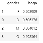
We can see the ratio of success, bogo, and discount on gender.
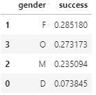
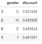
The difference between female and male is not much.
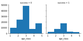
Now we review the histograms of success, bogo, and discount over age to see how we can combine age values into some compatible age classes for better prediction.
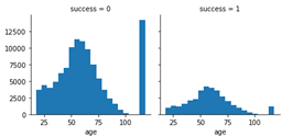
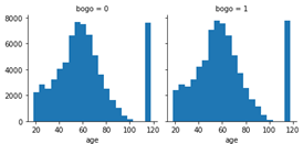
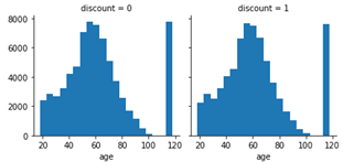
From these plots, we can set five classes of age:
[1, 2, 3, 4, 5] = [ < 30, < 50, < 75, < 85, rest ]
and we can see the distribution of success on age_class:
|
3 17623 2 7868 4 2876 1 2706 5 2506 Name: age_class, dtype: int64 |
|
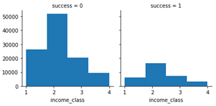
Similarly, we can create four income classes:
[1, 2, 3, 4] = [ < 50.000, < 80.000, < 100.000, rest]
From the column time_on, we can extract value year to check its effect on the ratio of success.
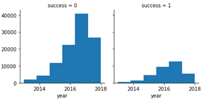
So, we extract year value from time_on and encode into columns to use in our dataframe.
After many steps of encoding and cleaning unnecessary data, we save the new data in the file pdata.csv.
Int64Index: 141515 entries, 0 to 306532
Data columns (total 26 columns):
# Column Non-Null Count Dtype
--- ------ -------------- -----
0 success 141515 non-null uint8
1 customer_id 141515 non-null int64
2 time 141515 non-null int64
3 offer_viewed 141515 non-null uint8
4 offer_id 141515 non-null uint8
5 time_on 141515 non-null datetime64[ns]
6 D 141515 non-null uint8
7 F 141515 non-null uint8
8 M 141515 non-null uint8
9 O 141515 non-null uint8
10 reward 141515 non-null uint8
11 min_spend 141515 non-null uint8
12 duration 141515 non-null uint8
13 mobile 141515 non-null uint8
14 social 141515 non-null uint8
15 web 141515 non-null uint8
16 bogo 141515 non-null uint8
17 discount 141515 non-null uint8
18 age_class 141515 non-null uint8
19 income_class 141515 non-null uint8
20 2013 141515 non-null uint8
21 2014 141515 non-null uint8
22 2015 141515 non-null uint8
23 2016 141515 non-null uint8
24 2017 141515 non-null uint8
25 2018 141515 non-null uint8
dtypes: datetime64[ns](1), int64(2), uint8(23)
Conclusion
After these steps of analyzing and processing the data relationship, from the supplied data, if Starbucks wants to have more success in offers bogo and discount, they need to concentrate on customers that are in:
- gender of female and male.
- age_class from 30 to 50.
- income_class from 50.000 to 80.000.
- Although the customers engaged in year 2017 had the most success offers, we can't conclude easily because the data of year 2018 is too small.
Separate data for bogo and discount training models
We need some adjustment to separate the data into two parts. For prediction model, we change time_on data type as int64, normalize data columns 'time', 'reward', 'min_spend', 'duration', and 'time_on'.
Now we are ready to create bogo and discount data.
# Seperate two instant dataframes for bogo and discount
bogo = data[data['bogo'] == 1]
discount = data[data['discount'] == 1]
# Save data into csv files
bogo.to_csv(DIR+'bodo.csv', index=False)
discount.to_csv(DIR+'dicsount.csv', index=False)
Prepare data for sklearn Logistic Regression models.
# Predict the success bogo, we delete unrelated rows
Y_bogo = bogo['success']
X_bogo = bogo.drop(axis=1,
columns=['discount', 'success',])
# Predict the success discount, we delete unrelated rows
Y_disc = discount['success']
X_disc = discount.drop(axis=1,
columns=['bogo', 'success',])
X_bogo.info()
X_disc.info()
By sklearn train_test_split, we create train set and test set for our models. We also use these train set and test for two local training models: Sklearn Logistic Regression and Autogluon Tabular
from sklearn.model_selection import train_test_split
from sklearn.linear_model import LogisticRegression
X1_train, X1_test, Y1_train, Y1_test = train_test_split(X_bogo,
Y_bogo, test_size=0.2, random_state=18)
X2_train, X2_test, Y2_train, Y2_test = train_test_split(X_disc,
Y_disc, test_size=0.2, random_state=18)
We can describe in the following workflow.
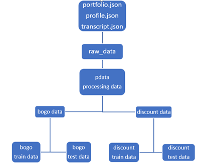
Data workflow
V. Train the models
The workflow of machine learning can be displayed in the following chart.
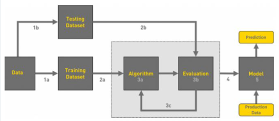
Overview of Machine Learning flowchart.
We deploy our training process through three steps.
1. Sklearn Logistic Regression models
The first bogo model.
bogo_clf = LogisticRegression(random_state=18, max_iter= 1000).fit(X1_train, Y1_train)
bogo_predictions = bogo_clf.predict(X1_test)
print('Train accuracy: ', bogo_clf.score(X1_train, Y1_train),
'\n---\nTest accuracy: ', bogo_clf.score(X1_test,
Y1_test))
We have the accuracy:
Train accuracy: 0.7852093624002933
---
Test accuracy: 0.7872102764590896
The second discount model.
disc_clf = LogisticRegression(random_state=18, max_iter= 1000).fit(X2_train, Y2_train)
disc_predictions = disc_clf.predict(X2_test)
print('Train accuracy: ', disc_clf.score(X2_train, Y2_train),
'\n---\nTest accuracy: ', disc_clf.score(X2_test,
Y2_test))
We have the accuracy:
Train accuracy: 0.751672091276512
---
Test accuracy: 0.7533619456366237
Very good results for sklearn Logistic Regression models.
2. Autogluon Tabular models on local
Now we adjust data a little bit for compatible Autogluon Tabular models.
# Set category type for category columns
X_bogo = pd.concat([Y1_train,X1_train], axis=1)
cat_cols = ['success', 'mobile', 'social', 'web', 'customer_id', 'offer_id',
'bogo', 'D', 'F', 'M', 'O', 'age_class', 'income_class', 2013, 2014,
2015, 2016, 2017, 2018]
X_bogo[cat_cols] = X_bogo[cat_cols].astype('category')
X_disc=pd.concat([Y2_train,X2_train], axis=1)
disc_cat_cols = ['success', 'mobile', 'social', 'web', 'customer_id', 'offer_id',
'discount', 'D', 'F', 'M', 'O', 'age_class', 'income_class', 2013, 2014,
2015, 2016, 2017, 2018]
X_disc[disc_cat_cols] = X_disc[disc_cat_cols].astype('category')
And now we are ready for training our bogo model.
from autogluon.tabular import TabularPredictor
bogo_predictor = TabularPredictor(label='success', problem_type='binary',
verbosity = 1).fit(X_bogo, presets='best_quality', time_limit=600)
We get the leaderboard, and sort the score_val values.
bogo_leaderboard = bogo_predictor.leaderboard(X_bogo, silent=True)
bogo_leaderboard['score_val'].sort_values(ascending=False)
We get such an impressive result:
15 0.980294
14 0.980294
13 0.980294
11 0.979893
12 0.979875
9 0.979579
10 0.979561
8 0.979160
6 0.978636
5 0.978636
4 0.978636
7 0.978287
3 0.970520
1 0.864556
0 0.863770
2 0.841272
16 0.781614
17 0.781544
Name: score_val, dtype: float64
With the test set:
bogo_predictor.evaluate(pd.concat([Y1_test,X1_test],
axis=1))
{'accuracy': 0.9773806199385646,
'balanced_accuracy': 0.952397164785564,
'mcc': 0.9323110209968879,
'roc_auc': 0.9914061353237994,
'f1': 0.945325683428957,
'precision': 0.9852268730214562,
'recall': 0.9085306519623743}
The accuracy is 97.74%, the minimum is recall 90.85% and the maximum is roc_auc 99.14%.
All the score results are much better than sklearn models ones.
Similarly, we train the discount model.
disc_predictor = TabularPredictor(
label='success', problem_type='binary',
verbosity = 1).fit(X_disc,
presets='best_quality', time_limit=600)
We get the leaderboard, and sort the score_val values.
disc_leaderboard = disc_predictor.leaderboard(X_disc, silent=True)
disc_leaderboard['score_val'].sort_values(ascending=False)
Result:
12 0.981008
11 0.981008
16 0.980972
15 0.980936
13 0.980918
9 0.980901
14 0.980865
10 0.980811
6 0.980132
5 0.980132
7 0.980132
8 0.979935
4 0.972978
0 0.856790
3 0.855431
2 0.838442
1 0.836761
19 0.788923
18 0.786938
17 0.786688
Name: score_val, dtype: float64
With the test set:
disc_predictor.evaluate(pd.concat([Y2_test,
X2_test], axis=1))
{'accuracy': 0.9828326180257511,
'balanced_accuracy': 0.9673226683523406,
'mcc': 0.9548884574734777,
'roc_auc': 0.9939625410074887,
'f1': 0.9654278305963699,
'precision': 0.9973214285714286,
'recall': 0.9355108877721943}
The accuracy is 98.28%, the minimum is recall 93.55% and the maximum is roc_auc 99.40%.
We get the very good results with Autogluon Tabular models on local model training processing.
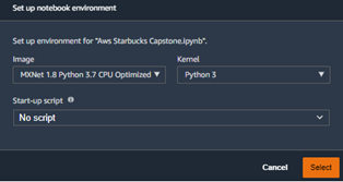
3. Autogluon with Aws Sagemaker
From Aws gateway, we run Amazon Sagemaker Studio. Because this project is executed with Autogluon Tabular prediction models, we must run our notebook on the most compatible instance type. We select the low cost instance type ml.t3.medium with suitable powerful kernel MXNet 1.8 Python 3.7 CPU Optimized.
According to the guide in Cloud Training with AWS SageMaker - AutoGluon and Cloud Deploying AutoGluon Models with AWS SageMaker, we implement as following:
1. Prepare python code and config file for entry points to create and deploy Autogluon Tabular TabularPredictor models:
a. ag_model.py
b. tabular_train.py
c. tabular_serve.py
d. config.yaml
2. Create data for bogo models. We get data from bogo.csv that we create from previous steps and use pandas sample to separate into train set and test set with the fraction 80% and 20%. From these data, we create compatible csv files to upload into our s3 bucket.
DIR = 'data/'
bogo = pd.read_csv(DIR + 'bogo.csv')
bg_train = bogo.sample(frac = 0.8, random_state = 18)
bg_test =
bogo.drop(bg_train.index)
bg_train_file = 'bg_train.csv'
bg_test_file = 'bg_test.csv'
bg_train.to_csv(bg_train_file,
index=False)
bg_test.to_csv(bg_test_file,
index=False)
train_input =
ag.sagemaker_session.upload_data(
path=os.path.join("data", "bg_train.csv"), key_prefix=s3_prefix)
eval_input =
ag.sagemaker_session.upload_data(
path=os.path.join("data", "bg_test.csv"), key_prefix=s3_prefix)
config_input = ag.sagemaker_session.upload_data(
path=os.path.join("config", "config.yaml"), key_prefix=s3_prefix)
Next we create AutoGluon tabular model:
from ag_model import (
AutoGluonTraining,
AutoGluonInferenceModel,
AutoGluonTabularPredictor,
)
ag = AutoGluonTraining(
role=role,
entry_point="tabular_train.py",
region=region,
instance_count=1,
instance_type="ml.m5.2xlarge",
framework_version="0.3.1",
base_job_name="autogluon-tabular-train",
)
We create training job and train our bogo model:
job_name =
utils.unique_name_from_base("autogluon-sm")
ag.fit(
{"config": config_input, "train": train_input, "test": eval_input},
job_name=job_name,)
In the config file, it set time_limit = 600 (second), then after successfully training, we get the message:
2022-01-10 16:13:58 Completed - Training job completed
Training seconds: 907
Billable seconds: 907
We have another training with no time_limit, it takes much time:
2022-01-10 17:30:14 Completed - Training job completed
Training seconds: 4052
Billable seconds: 4052
When comparing the metrics score, we see the differences are very small. We can conclude time_limit = 600 is enough for our data with low cost.
After training, we prepare a little bit of data for deploying the model. We copy the model image model.tar.gz to the data directory of the endpoint:
s3_deploy = f"ag_sm_deploy/{utils.sagemaker_timestamp()}"
output_path = f"s3://{bucket}/{s3_deploy}/output/"
endpoint_name =
sagemaker.utils.unique_name_from_base("sg-ag-deploy")
# Copy model image to
endpoint data directory
!aws s3 sync s3://sagemaker-us-east-1-503563512855/autogluon-sm-1641831565-ea74/output/ s3://sagemaker-us-east-1-503563512855/sg-ag-deploy-1641837746-719b/models
We setup the process to deploy the endpoint:
instance_type = "ml.m5.2xlarge"
model =
AutoGluonInferenceModel(model_data=model_data,
role=role,
region=region,
framework_version="0.3.1",
instance_type=instance_type,
entry_point="tabular_serve.py",)
bogo_predictor =
model.deploy(initial_instance_count=1,
serializer=CSVSerializer(),
instance_type=instance_type)
We prepare test data for our bogo model.
bg_test_data =
pd.read_csv('data/bg_test.csv')
bg_success =
bg_test_data.loc[1:,0].tolist()
bg_success = [int(item) for item in bg_success]
bg_test_data.shape
(14324, 25)
There are 14.324 test data rows. We try a test prediction of 500 data test row:
bg_test_data.drop(columns=['mobile', 'bogo', 'discount','success'], axis=1,
inplace=True)
bg_predictions =
bogo_predictor.predict(bg_test_data[:500].values)
bg_predictions[:5]
[[0.0, 0.9517540335655212, 0.04824599251151085],
[1.0, 0.008261322975158691, 0.9917386770248413],
[0.0, 0.9948185682296753, 0.005181452259421349],
[1.0, 0.008979439735412598, 0.9910205602645874],
[0.0, 0.9975728392601013, 0.0024271896108984947]]
The endpoint execution can't response to the large test data timeout problem, so we write some code to get the result of all test data predictions.
NUM_TEST = bg_test_data.shape[0]
SEGMENT = 500
ITER = NUM_TEST //
SEGMENT
bg_preds = []
for k in range(ITER):
preds=bogo_predictor.predict(bg_test_data[k*SEGMENT:(k+1)*SEGMENT].values)
bg_preds.extend(preds)
preds =
bogo_predictor.predict(bg_test_data[ITER*SEGMENT:].values)
bg_preds.extend(preds)
bg_predictions = [int(item[0]) for item in bg_preds]
Using sklearn metrics to get the prediction metric scores from our prepared data bg_predictions and bg_success.
from sklearn.metrics import (accuracy_score,
f1_score, balanced_accuracy_score,
precision_score, recall_score, roc_auc_score)
print('Bogo predictions test
scores',
'\naccuracy_score: ',
accuracy_score(bg_predictions, bg_success),
'\nbalanced_accuracy_score:
',
balanced_accuracy_score(bg_predictions, bg_success),
'\nprecision_score: ',
precision_score(bg_predictions, bg_success),
'\nrecall_score: ',
recall_score(bg_predictions, bg_success),
'\nf1_score: ',
f1_score(bg_predictions, bg_success),
'\nroc_auc_score',
roc_auc_score(bg_predictions, bg_success))
Bogo predictions test scores
accuracy_score: 0.9867346226349228
balanced_accuracy_score: 0.9891488181708774
precision_score: 0.945617402431222
recall_score: 0.9932795698924731
f1_score: 0.9688626679777124
roc_auc_score 0.9891488181708775
The accuracy is 98.67 %, the minimum is precision 94.56% and the maximum is recall 99.33%.
3. Similarly, we create our discount Autogluon tabular model and get the same results reference to my notebook my_Starbucks_Capstone.ipynb.
Discount predictions test scores
accuracy_score: 0.9851931330472103
balanced_accuracy_score: 0.9890291251091365
precision_score: 0.9451631046119235
recall_score: 0.9964423361992292
f1_score: 0.9701255592437581
roc_auc_score: 0.9890291251091367
The accuracy is 98.52 %, the minimum is precision 94.52% and the maximum is recall 99.64%. We write some code to plot these scores to have more interesting results.
metric = ['accuracy_score', 'balanced_accuracy_score', 'precision_score',
'recall_score', 'f1_score', 'roc_auc_score']
disc_score =
[accuracy_score(disc_predictions, disc_success),
balanced_accuracy_score(disc_predictions, disc_success),
precision_score(disc_predictions, disc_success),
recall_score(disc_predictions, disc_success),
f1_score(disc_predictions, disc_success),
roc_auc_score(disc_predictions, disc_success)]
df =
pd.DataFrame.from_dict({'metric': metric, 'score': disc_score})
df
x,y = df['metric'], df['score']
plt.scatter(x, y, c=['r' if k<.95 else 'b' for k in y ])
plt.axhline(y=0.95, color='g', linestyle='--')
plt.ylim(bottom=.4,top=1.02)
# Add labels
plt.ylabel("Scores")
# plt.suptitle("Bogo
Test Scores", size=14)
plt.title("Discount Test
Scores", size=10)
# Give it some pizzaz!
plt.style.use("Solarize_Light2")
plt.gcf().autofmt_xdate()
plt.show()
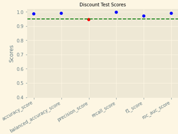
Very impressive scores. These scores prove that our Autogluon tabular are the most effective models for these problems.
4. Research
When researching on the Internet, there was a paper solved the same problem with ours, and the author implemented on three models, he got the results as following:
The author got the scores from three models.
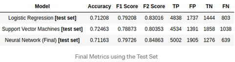
Starbucks Capstone Project Stephen Stephen Blystone | Medium
VI. Conclusion
1. We examine and analyze three json files to combine a useful related data.
2. We can see the ratio success offers from customers with details in gender, age classes, income classes.
3. We separate our data into two distinct parts for two prediction models of bogo and discount offers.
4. We implement successful Sklearn Logistic Regression Models and train them to get the good accuracy score about 78% and 75%
5. We implement successful Autogluon Tabular Models on local and train them to get the very impressive results about 98% (the above results).
6. We implement successful Autogluon Tabular Models on Aws Sagemaker and train them to get the very impressive results about 98% (the above results).
7. Autogluon Tabular Model is much better than Sklearn Logistic Regression Model. Autogluon Tabular Model is the most effective model for these similar problems.
VII. Improvement
1. We can examine if informational data has an effect on other offers.
2. We can use unsupervised model to prepare our data more effective to get more interesting results about various classification of customers combining gender, age, income, time to become member.
3. We can use other compatible machine learning models to learn more with these wonderful datasets.
VIII. References
1. Propensity model.
2. Sklearn Logistic Regression.
4. Deploying AutoGluon Models with AWS SageMaker.
5. Code-free machine learning: AWS Machine Learning Blog.
6. AutoGluon Tabular with SageMaker Examples.
7. Cloud Training with AWS SageMaker - AutoGluon.